Precision Timing Meets Detector Development: Collaboration with Laser Components

作者 Catherine Cruz Luukkonen | 日期 20 May 2026

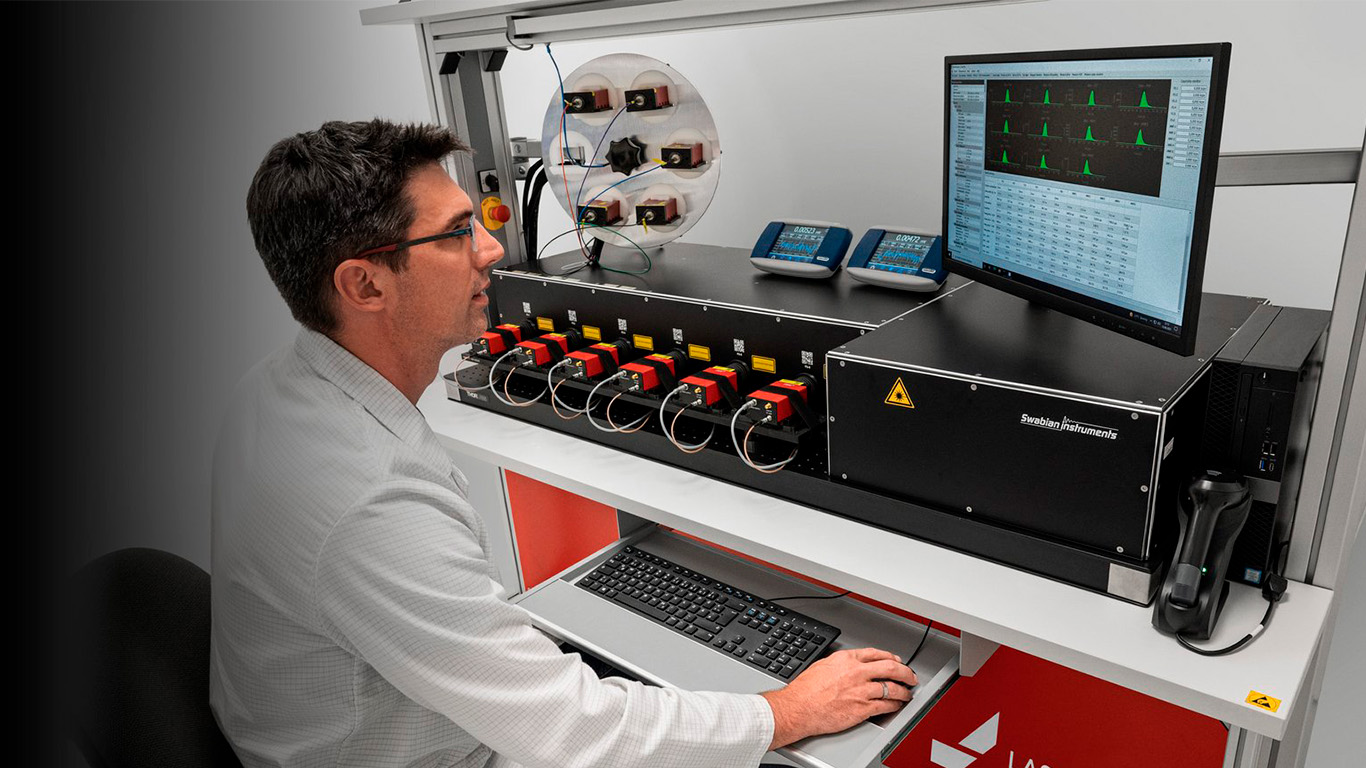
Testing COUNT® series SPAD detectors for photon-counting applications

We are happy to share more about our collaboration with LASER COMPONENTS, a high-tech optoelectronics company specializing in detectors, emitters, fiber optics, and optical components. Together, we’ve built a powerful testing setup that combines the LASER COMPONENTS COUNT series SPAD detector with our high-precision Time Tagger Ultra.

Detectors are a vital component of the measurement system, as the processed signal depends on the sensitivity, accuracy, response time, and reliability of this device under different conditions. So it is of key importance to understand the detector as well as every other component in the measurement system.

To characterize a detector, there are a few key aspects that need to be taken into account: timing jitter, dark count rate, dead time and afterpulsing, and photon detection efficiency (PDE). All of these share a crucial requirement: precise timing is essential to measure and understand these specifications as accurately and realistically as possible.

The Time Tagger Ultra allows a complete characterization of the SPAD detectors. This Time-to-Digital Converter timestamps events with a very high resolution (down to 8 ps), with a precision in the order of picoseconds, making a complete characterization of the SPAD detectors possible. With up to 18 available channels, it supports simultaneous measurements from up to 4 lasers and up to 12 SPAD detectors, allowing efficient parallel characterization without compromising accuracy.

This integrated system enables precisely calibrated detector testing facilities designed for a wide range of photon-counting applications, including LiDAR, fluorescence lifetime techniques, and photonic quantum technologies.

A person using the laboratory workstation showing a detector characterization setup on a ThorLabs optical bench. The rack contains six COUNT detector modules with fiber connections, flanked by a Swabian Instruments Time Tagger Ultra unit. Two small display monitors sit on top of the rack, and a computer monitor displays timing histograms. A circular mount holding several detectors is visible on the left, and four laser driver modules are mounted on the upper rail. — Detector characterization setup, featuring a Swabian Instruments Time Tagger Ultra (right) as the central timing element, alongside COUNT detector modules.

To make the workflow seamless, the system is paired with our intuitive and flexible software, enabling:

Fast configuration of test routines
Real-time visualization and performance monitoring
Reproducible measurement protocols and standardized reporting
Effortless handling of multi-detector, multi-laser datasets

Using the Time Tagger Ultra as the central timing acquisition and analysis platform, the following performance metrics of COUNT® series detectors are characterized under reproducible, calibrated conditions:

Timing jitter: precision in event timing

The timing jitter is the uncertainty in the registered detection time with respect to the instant at which the event actually occurs. It sets a fundamental limit on the temporal resolution of the measurement, since larger jitter directly degrades the ability to resolve fast dynamics or distinguish events that are close in time.

To determine the timing resolution, both a start reference and a stop signal are required. In this measurement, the start reference is given by the laser synchronization output, while the stop signal is provided by the detector output pulse. The laser sync and detector signals are connected to two separate input channels of the Time Tagger. A timing measurement is then performed by recording the time delay between the start and stop signals over many repeated events. By configuring a sufficiently small bin width (down to 1 ps) and collecting a large number of counts, a high-statistics time-delay histogram can be obtained.

The timing jitter is extracted by quantifying the width of the histogram peak, which represents the overall timing uncertainty of the measurement chain. This includes contributions from all relevant components, such as the Time Tagger itself, the laser synchronization signal, and the laser pulse duration. In this work, the jitter is reported as the RMS timing jitter, obtained by calculating the standard deviation of the peak:

\sigma_{measurement} = \sqrt{2\sigma_{TT}^2 + \sigma_{pulse}^2 + \sigma_{sync}^2}

Where:

\begin{aligned} \sigma_{TT} &= 8 \text{ ps} \\ \sigma_{pulse} &= 40 \text{ ps} \\ \sigma_{sync} &= 30 \text{ ps} \end{aligned}

And this gives a timing jitter of the whole system of $\sigma_{measurement} \simeq 50 \text{ ps}$

Dark count rate: counting noise when the signal is off

Dark counts are false detection pulses generated in the absence of incident photons. This leads to decreased sensitivity to weak signals and results in an inconveniently high signal-to-noise ratio.

The dark count rate $R_{dc}$ is calculated by counting the number of photon arrivals $N_p$ recorded by the Time Tagger on the detector channel during the acquisition time $\Delta T$ :

R_{dc} = \frac{N_p}{\Delta T}

With the Time Tagger’s built-in count-rate tools, dark count rate measurements can be performed continuously, logged automatically, and compared across multiple detectors in parallel. This makes it straightforward to screen detectors, monitor stability over time, and directly evaluate the impact of operating parameters such as temperature or bias voltage on the dark count rate.

Dead time and afterpulsing: recovery behavior under high rates

After each detection event, photon-counting modules require a reset period during which further events cannot be registered (dead time). During this time, incoming photons are not captured by the detector, potentially leading to undercounting if the dead time is significant. COUNT® modules exhibit a fixed dead time defined by their reset circuitry. Beyond this interval, time-correlated false events may occur due to afterpulsing, which is typically caused by the release of trapped charge following an avalanche.

Both effects are quantified by recording an autocorrelation histogram of the detector output signal. The dead time appears as an empty region at short time differences, since the detector is unable to register any additional events immediately after a detection. Once the dead time region is passed, the histogram should approach a constant baseline level corresponding to uncorrelated events. Any additional counts observed above this baseline indicate afterpulsing, and its probability is obtained by integrating the excess counts within a defined time window after the dead time.

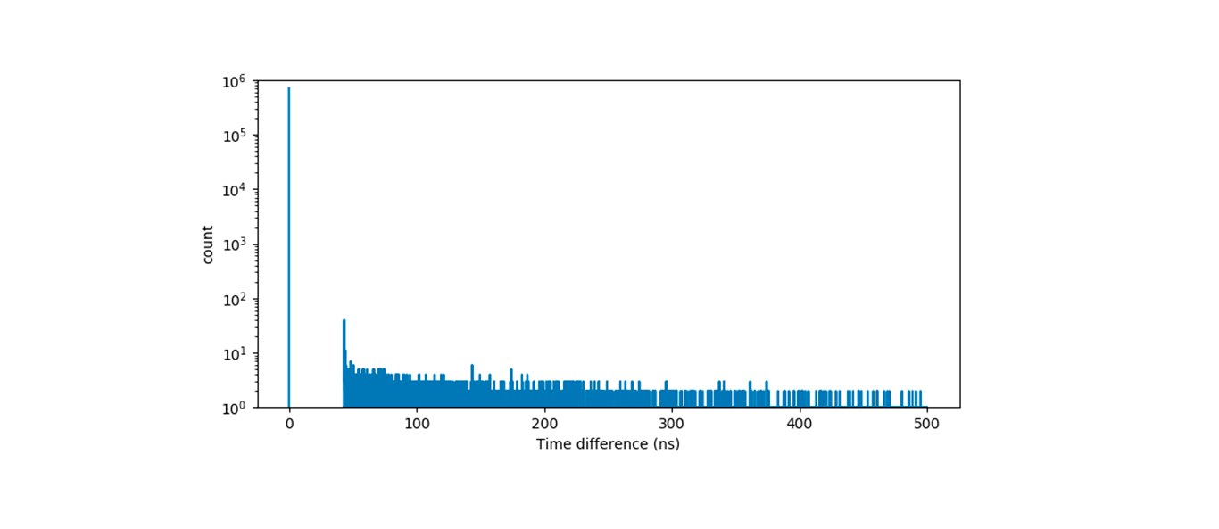
Bar chart showing the distribution of time differences in nanoseconds on a logarithmic count scale. A dominant spike near 0 ns reaches approximately 10⁶ counts, and a secondary cluster of bars appears between roughly 40–500 ns, with counts ranging from about 1 to 40. The y-axis (COUNT) uses a logarithmic scale from 10⁰ to 10⁶, and the x-axis spans 0 to 500 ns. — Autocorrelation histogram of the detector output. The zero-delay bin corresponds to the total number of recorded events, while the remaining bins represent event pairs separated by up to 500 ns. No counts are observed below 42 ns due to the COUNT® module dead time.

With the information provided by the histogram, it is possible to calculate the afterpulsing probability as the ratio between the number of pulses $N_{ap}$ that are separated in time at 500 ns maximum $(N_1 \ldots N_m)$ and the total number of pulses recorded $N_\Sigma = N_0$ :

P_{ap} = \frac{N_{ap}}{N_\Sigma} = \frac{\sum_{i=1}^{m} N_i}{N_0}

Photon detection efficiency (PDE): from photons to counts

PDE describes the probability that an incident photon generates a valid output pulse. It is determined as the ratio of the corrected detection rate to the incident photon rate. Since the required optical power is typically below the sensitivity of standard power meters, the laser power is monitored using a beam-splitter reference channel, and the conversion factor is calibrated using a calibrated power meter. This enables accurate and traceable determination of the photon rate at the detector input.

By combining robust hardware with powerful software, this collaboration helps ensure superior detector performance, quality, and reliability for accurate characterization in both research and industrial settings. The Time Tagger provides the timing precision, multi-channel scalability, and stability needed to extract key detector metrics such as timing jitter, dark count rate, dead time, afterpulsing, and photon detection efficiency in a reproducible way. This not only simplifies detector evaluation and comparison, but also supports long-term monitoring and quality control, ensuring that detector performance can be trusted over time and across different measurement environments.

For more information, please contact solutions@swabianinstruments.com.