Multichannel Continuous Histogramming: Advancing Fluorescence Lifetime Flow Cytometry with Melissa Skala’s Team and Swabian Instruments

| 日期 07 October 2025

Scientific Background: Fluorescence Lifetime Flow Cytometry

Flow cytometry is a powerful technique for single-cell analysis, usually based on measuring the brightness of a label to distinguish between cell types or functional conditions, such as evaluating health conditions and protein expression levels. By introducing time-resolved photon counting to traditional flow cytometry setups, researchers achieve a new axis of information, Fluorescence Lifetime Flow Cytometry (FLFC), providing insights into cell microenvironments. The distinct fluorescence-decay times, characteristic of specific fluorophores, enable precise discrimination even with weak signals or when emission spectra overlap.

Single Photon Counting Techniques for Bioimaging Applications in the Skala Group

Dr. Melissa Skala is a renowned bioimaging scientist, a professor at the University of Wisconsin-Madison (UW), and an investigator at the Morgridge Institute for Research. Skala’s group has extensive experience with various imaging techniques and the incorporation of time-correlated measurements.

Key Takeaways and Impact

When PhD researcher Adrian Abazi set out to improve the resolution of Time-of-Flight (ToF) LiDAR at the University of Münster, he and his team faced a familiar challenge: traditional timing electronics weren’t precise enough. Older systems added noise, slowed workflows, and required heavy post-processing, limiting how far they could push their experiments.

One example is their detailed GitHub repository that documents the design of their time-resolved single-photon detection system built for flow cytometry and fluorescence lifetime analysis. The core innovation lies in using timestamped photon counting to go beyond the limitations of conventional frequency-domain techniques with modulated excitation and analog detection or time-domain techniques with gated detection schemes. Using the Swabian Instruments Time Tagger Ultra as the data acquisition unit, they demonstrated a simplified hardware architecture (fewer custom electronics), improved software processing (data logged as text or processed in Python via the Time Tagger API), and easier integration (direct connection to single photon detectors such as SPADs or PMTs). The Time Tagger is able to acquire and analyze the signal directly from detectors such as PMTs used in this project. Having the time domain data from the Time Tagger as a continuous stream of millisecond-integrated decay histograms was crucial to resolving the stages of a single cell traversing the laser spot based on fluorescence photon count fluctuations and aggregating photons to reconstruct the single-cell fluorescence decay ¹. Moreover, the flexibility of time-tagged data supports virtual gating and retrospective analysis, helping to further identify previously unrecognized cell populations or dynamic features of rare events. This level of detail could significantly enhance applications such as rare cell detection, multi-parametric immunophenotyping, or single-molecule counting. Additional applications for this methodology include the investigation of NAD(P)H and FAD autofluorescence lifetime as a proxy for metabolic state, FRET-based biosensors for protein–protein interaction mapping, and pH, viscosity, and ion sensing using environment-sensitive dyes ^{2 3}.

The Time Tagger’s software engine has been crucial for these developments and lays the foundation for upcoming advances within the analysis side. One recent development in the collaboration between Dr. Skala’s group and Swabian Instruments has been spearheaded by Dr. Kayvan Samimi and Dr. Amani Gillette, experts in time-resolved flow cytometry measurements for label-free immune cell imaging applications, among other bioimaging work.

Experimental Setup for Fluorescence Lifetime Flow Cytometry and Challenges

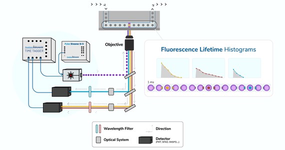
Prof. Melissa Skala’s Fluorescence Lifetime Flow Cytometry (FLFC) workflow can be summarized as follows:

1. Measure for a certain time T_m (Figure 1 shows 1 ms per frame) shorter than the passage of a single cell through the laser beam.

2. After time T_m, evaluate if photon flux is above the background level and if there is a cell in the detection volume (yes/no). This step can be performed using either the histogram measurement or a counter; the goal is to determine whether a cell is flowing through the detection volume or not.

3. If no cells are detected, the measurement is no longer necessary and can be discarded. In this case, the histogram or collected counts can be deleted entirely, as the data collected is basically an empty (background) measurement.

4. New measurements are constantly being taken in T_m intervals, regardless of the content. Based on fluorescence content, the cells are filtered and combined. Initially, a 10-ms TimeDifferences measurement class consisting of 10 consecutive 1-ms histograms was used, analyzed, and repeated in a loop every 10 ms. In Figure 1, the first frame with “yes” is the first non-empty histogram that includes counts, which is acquired. Then the measurement is continued for intervals with t = T_m, until the next “no.”

5. If multiple consecutive events are identified, the histograms are kept. This serves as a filter for artifacts based on the knowledge that a cell needs more than two consecutive time steps (2x T_m) to be able to travel through the detection volume (2 ms for Figure 1 setup).

6. If there are histograms without events, the process is stopped (the cell has cleared the detection volume).

7. Multiple histograms are merged into one large histogram for fluorescence lifetime calculation, referred to as “combined decay histogram for each single cell transit event” (Figure 1).

8. User-specific follow-up tasks can be made from the merged histogram, including lifetime estimation or phasor analysis, etc.

In previous experimental setups, Dr. Samimi implemented a Python programming code using the Swabian Instruments API, where startFor() and waitUntilFinished() were executed multiple times consecutively, a standard program flow in conventional approaches. However, the limitation was that both start and stop instructions were not immediately executed due to the intrinsic time associated with the programming processors, causing a blockage in the thread, resulting in a measurement deadtime. Specifically, the startFor() method blocks a thread for approximately 4 microseconds, which could be considered negligible given the timing scale of the overall experiment. On the other hand, waitUntilFinished() blocks the thread for around 20,000 - 50,000 microseconds, or 20-50 ms, depending on the computational speed and capabilities of the PC in the setup. This corresponds to approximately 50 frames in the flow cytometry application, resulting in a significant amount of dead time.

Skala group’s interest in this project relied on capturing complete cells with a transition time of around 4 to 5 ms (Figure 1). Due to the long blockage caused by waitUntilFinished(), the approach was not ideal, as many cells were missed while waiting for the processor to finish; therefore, an initial compromise was made. In this case, the temporary “band aid solution” was to measure one histogram over a “long” integration time (twice as long as a cell transit of 5 ms):

Measurement time = 10 ms
startFor(10 ms) 
waitUntilFinished()

So the total time for one measurement is:

startFor() =          4 microseconds 
Measure =             10 000 microseconds 
waitUntilFinished() = 20 000 microseconds 
Total:                30 004 microseconds 
Desired:              10 000 microseconds 
                      Acceptable since any 10 ms window will most likely either contain zero or one cell in it. 

                      1 000 microseconds 
                      Even more desirable because with the finer resolution, one can capture the travel of a single cell through the detection volume 
                      and avoid including background photons in the aggregated histograms. 
                      This results in improved signal-to-background ratio in the measured cell decays.

The initial implementation required a 10-ms TimeDifferences measurement class consisting of 10 consecutive 1-ms histograms. The 10 ms measurement would be read, analyzed, and repeated loop. With the waitUntilFinished() overhead, that resulted in 10ms/30ms or <33% duty cycle, not a desirable outcome.

Innovation in the Implementation of a MultiChannelContinuousHistogram() Class for Faster Experimental Outcomes

Following an insightful conversation at Photonics West 2025 and a subsequent collaboration, a solution was identified to avoid using the waitUntilFinished() approach. This solution is implemented via a CustomMeasurement(), coined MultichannelContinuousHistogram().

The idea behind MultichannelContinuousHistogram() is that it starts the measurement similar to startFor(), then enables the collection of multiple histograms within defined intervals. For the case of Figure 1, it is now possible to work with the goal of 1 ms instead of 10ms. In addition to this, MultichannelContinuousHistogram() is also able to introduce the binary logic that determines whether there are cells, and as a consequence either discards or merges multiple 1 ms histograms into a single histogram with a time frame that can be adjusted based on the cell requirements (in this case, 4-5 ms duration). Once the entire sample run is finished, the method is finalized and can be closed with waitUntilFinished() without suffering from the blockage limitation.

With this approach, one can seamlessly perform the following implementation and include many more measurements, and the “waitUntilFinished()” function only requires being called once, this method significantly increases the recovery of cell events, increasing the active measurement duty cycle from ~30% in the original implementation to ~93% (achieved in Python, limited only by the processing code).

Measure time = 1 ms

startFor() # or start() → can be running for minutes or hours theoretically

1 ms measurement # no cell, discard
1 ms measurement # no cell, discard
1 ms measurement # cell, keep
1 ms measurement # cell, keep
1 ms measurement # cell, keep
1 ms measurement # no cell, discard this measurement and merge the previous 3
1 ms measurement # no cell, discard
1 ms measurement # no cell, discard
1 ms measurement # cell, keep
1 ms measurement # cell, keep
1 ms measurement # cell, keep
1 ms measurement # cell, keep
1 ms measurement # no cell, discard this measurement and merge the previous 4

waitUntilFinished()

Overall, this relatively straightforward but meaningful approach sets a foundation for further developments in Fluorescence Lifetime Flow Cytometry (FLFC) experiments with high timing resolution.

This project, in particular, was not focused on cell sorting capabilities, which is why the data collection could occur for such a long time without calling the waitUntilFinished() method. For projects that may consider adding the capability of cell sorting, the process could be implemented by:

startFor() # or start()
1 ms measurement # no cell, discard
1 ms measurement # no cell, discard
1 ms measurement # cell, keep
1 ms measurement # cell, keep
1 ms measurement # cell, keep
1 ms measurement # no cell, discard this measurement and merge the previous 3, and stop the process
waitUntilFinished()

Then the cell sorting task would be implemented, and a new round of measurements would be resumed. The cycle would be repeated as many times as needed and would benefit from a more precise result than a conventional Histogram approach, given that the measurement interval could still be shortened to a 1 ms range instead of the 10 ms approach used in the past.

Future Work in Fluorescence Lifetime Flow Cytometry in the Skala Group

To summarize, timestamped Fluorescence Lifetime Flow Cytometry (FLFC) leverages differences in fluorescence decay times to investigate cells beyond what is feasible with standard setups. Dr. Kayvan Samimi’s work within Prof. Melissa Skala’s group at UW is fundamental for the advancement of the field and pushes the boundaries of what’s possible. Dr. Amani Gillette is working to commercialize a label-free flow-cytometry system capable of early prediction of fit-for-purpose T cell therapy products using this methodology. Their challenges with timing sparked an additional layer to the preexisting work with Swabian Instruments and resulted in improved measurement capabilities. By reworking the conventional approach for histogramming cell detection when flowing through an illuminating spot with Swabian Instruments’ MultichannelContinuousHistogram() approach, the time resolution of the setup has been further optimized to capture complete cells while ensuring the experiment duration is not compromised, thereby accelerating developments in fluorescence lifetime flow cytometry applications.

Direct Quote

“Working with Swabian has been critical to the success of this fluorescence lifetime flow cytometer because we have tight timing requirements for photon histogramming and data streaming. We were excited to see the Time Tagger technology develop and work with Swabian to meet our specific needs for this application.”
— Dr. Melissa Skala

If you’re interested in expanding flow cytometry capabilities to incorporate the timing aspect and perform Fluorescence Lifetime Flow Cytometry experiments, we’re here to help!

References