卫星激光测距(SLR)与激光雷达(LiDAR):高精度遥感解决方案

什么是卫星激光测距(Satellite Laser Ranging, SLR)与激光雷达(Light Detection and Ranging, LiDAR)?
卫星激光测距(SLR)与激光雷达(LiDAR)是基于激光的遥感技术,已成为大地测量学、地球观测、地形测绘、林业、城市建模及自主系统等众多科技与工程领域的核心技术。脉冲激光源与精准时序电子设备的发展,使得高精度测量激光脉冲经远距离目标反射后的飞行时间(TOF,) 成为可能,并可利用光速c及往返路径修正因子,通过公式 将飞行时间转换为距离d。
LiDAR最早于1930年由 E. H. Synge 提出,最初作为大气光学探测工具,如今已发展为机载与地面系统。其通过发射高速激光脉冲、测量飞行时间,将反射信号转化为地理参考三维点。扫描形成的密集点云可区分地面、植被与人工建筑,适用于地形测绘、地表变化监测、基础设施建模及自主系统感知 1.
SLR则走上了不同的发展路径。20世纪60年代,美国国家航空航天局(NASA)的早期实验验证了其短距离应用可行性,随后将该方法拓展至轨道卫星测量 2。现代SLR系统依赖超快、低抖动的时序电子设备,为大地测量与空间科学任务提供毫米级测距精度 3。SLR通过地面站向搭载角反射器的卫星发射激光脉冲,除测距外,还可用于国际地球参考框架(ITRF)建立、地球重力场变化研究及卫星任务校准等关键测量工作。
尽管SLR与LiDAR的任务目标和工作尺度存在差异,但二者均依赖高精度、高稳定性、高速率的时序电子设备,以在严苛条件下输出稳定、高质量的测量结果。
SLR 与 LiDAR 的核心差异如表1所示4:
| 特征 | 卫星激光测距(SLR) | 激光雷达(LiDAR) |
|---|---|---|
| 主要应用 | 卫星定位跟踪,用于大地测量与轨道确定 | 地形测绘、植被分析及基础设施建模 |
| 测距范围 | 超远距离(最远可达 20,000 千米) | 短至中距离(机载/地面平台最远可达数千米) |
| 测量目的 | 监测地球形状、自转及重力场 | 生成地表特征的高精度三维模型 |
| 搭载平台 | 地面观测站,向轨道卫星发射激光 | 机载平台(向地面目标发射激光)、地面车辆(自动驾驶汽车) |
在实际应用中,二者的差异更为显著。在卫星激光测距领域,海洋测高任务通过地面激光测距优化精密轨道确定,支撑全球海平面研究;
在激光雷达领域,探测器与时序电子设备层面TOF测量精度的提升,实现对远距离目标更精准的测距 5.
时序电子设备与时间相关单光子计数在SLR和LiDAR中的作用
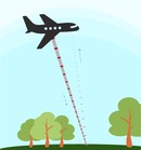
上文图1展示了SLR与LiDAR测量的典型装置。两种技术中,发射器均发射短激光脉冲;经过千米级传输与路径损耗后,接收器处的回波信号通常处于光子计数模式(每次发射的平均探测光子数远小于1)。单光子探测器(如单光子雪崩二极管SPAD、雪崩光电二极管APD、超导纳米线单光子探测器SNSPD或工作于光子计数模式的光电倍增管PMT)将每个探测到的光子转换为电脉冲,时间数字转换器(TDC)为该电脉冲打上时间戳,用于TOF估算。
数字脉冲发生器用于协调实验流程:触发激光器、控制探测器门控的开启与关闭,并为TOF测量提供“开始”信号,而探测器脉冲则作为一个或多个“停止”事件。TOF通过“开始”信号与一个或多个“停止”信号计算得出。生成的时间戳随后从TDC传输至计算机,进行数据评估。
在SLR的应用场景中,目标的大致距离是预先已知的,因此探测器采用距离门控模式,仅在预计回波到达时启动探测。图2a展示了典型测量结果:对卫星进行数秒跟踪后,在测量范围内的卫星距离处可观察到更高的点云密度。
在LiDAR的应用场景中,TDC记录每次“开始”信号后一个时间窗口内的所有“停止”事件,直至下一个激光脉冲发射。汇总并累加多次发射的数据,可得到TOF(或距离)相关的多“停止”事件直方图:如图2b所示,不同峰值对应高反射率表面(如植被冠层、地面、水面)。短时间范围内的强度凹陷由探测器与时序电子设备的死时间导致[1]。峰值宽度对应的可达距离分辨率由仪器响应函数(IRF)决定,该函数是激光脉冲宽度、探测器抖动与 TDC 计时抖动的卷积结果。

影响测量精度的各类计时参数汇总于表 2。
| T核心时间参数 | 对测量结果的影响 |
|---|---|
| 更窄的激光脉冲宽度(典型值:数十ps) | 距离分辨率更优(典型值:约mm级) |
| 更低的激光脉冲重复频率(典型值:kHz,对应时间尺度为ms) | 目标距离更远(SLR)或非模糊测量范围更大(LiDAR)(典型值:约km级) |
| 更低的 TDC 与探测器计时抖动(典型值:约10 ps/100 ps至ns级) | 距离分辨率更优(典型值:mm-cm级) |
| 更低的 TDC 与探测器死时间(典型值:ns级) | 信号动态范围更高、线性度更优 |
激光测距的常见挑战及时序电子设备与信号发生器的要求
表2所列的装置参数对时序电子设备提出了高要求,以实现SLR与LiDAR测量的毫米级精度。传统时序电子设备通常面临以下几方面挑战:
时间抖动: 要实现毫米级测距,TDC的固有抖动需控制在皮秒量级,避免对TOF估算引入显著误差(经验法则:1 ps约对应0.15 mm单程距离)。由于探测器的性价比通常更高,让TDC对系统时间抖动的贡献仅占探测器抖动的一部分,是更高效的设计方案。
死时间: 死时间应与探测器的恢复时间(典型值为纳秒级)相当或更短,确保在高计数率下不遗漏探测器响应信号、不扭曲测量结果,使多停止事件直方图在全动态范围内保持准确。
数据传输速率: 光子计数LiDAR 可能产生高总事件率;SLR的平均事件率通常低得多,但窄距离门控与突发回波仍要求TDC具备稳定的内部缓冲功能,避免在接收窗口内丢失时间戳。因此,两种场景均对TDC与计算机之间的持续无丢失数据传输提出严格要求,以防止时间戳丢失和测距统计结果偏差。
数据处理与分析: 传统计时系统常采用突发式文件写入方式,缓冲能力有限,且实时直方图绘制或TOF拟合功能不足。在高事件率下,这可能导致时间戳丢失和 I/O 暂停,进而造成数据处理与验证偏差。校准数据、门控时序和时钟元数据常存储于独立日志中,使得实验流程难以复现,数据难以快速重新分析。这会延长研发周期、增加运营成本,并降低在快速发展的科研或工业环境中的适应性。
复杂实验的流程协调: 传统计时系统很少提供统一控制平台,用于协调激光触发、探测器门控/ 距离窗口、扫描仪及TDC采集等环节。SLR与LiDAR需要具备高分辨率、低抖动及同步多通道输出功能的数字脉冲发生器,以控制所有组件,确保实验的可重复性。
Swabian Instruments - 施瓦本仪器的Time Tagger与Pulse Streamer提供SLR与LiDAR的先进解决方案
Swabian Instruments - 施瓦本仪器的Time Taggers系列产品与Pulse Streamer 8/2 兼具卓越精度与易用性,可实现高分辨率时间戳记录与实时数据访问,且系统复杂度低、额外开销小。与此同时,Pulse Streamer可实现数字与模拟输出信号的精准可编程控制,是同步激光脉冲、实现纳秒级分辨率探测器门控的理想选择。
SLR与LiDAR测量受益于Swabian Instruments - 施瓦本仪器Pulse Streamer 8/2的原因:
高时间精度: 数字脉冲波形的RMS时间抖动低于50 ps,分辨率达1 ns,为脉冲激光系统控制及SLR与LiDAR实验流程协调提供核心支持。
易于部署: 通过直观编码方式,可快速设计任意复杂度的数字脉冲图案与模拟波形,大幅简化部署流程。
便捷的实验控制: 配备本地库与专属图形化界面(GUI),可实现无缝实验控制。此外,Swabian Instruments - 施瓦本仪器还提供Pulse Streamer专用GUI,适用于测试场景与简单脉冲图案编程。
原生同步运行: 数字与模拟输出全程保持完全同步,无需进行跨设备的时间调整。
灵活部署: 支持以太网连接,可从任意位置远程控制,设备摆放更灵活。
SLR与LiDAR测量受益于Swabian Instruments - 施瓦本仪器Time Tagger的原因:
高时间分辨率: 仪器抖动低至1.5 ps RMS,对应测距误差与测量分辨率约0.2 mm。目前市售探测器的时间抖动至少高出一个数量级,因此系统整体仪器响应函数(IRF)主要受探测器限制,而非TDC限制。
超短死时间: Time Tagger X的死时间仅1.5 ns,且支持多事件探测模式,速度优于市售单光子探测器。该特点可确保捕获间隔极近的光子探测事件,无信号遗漏。
高数据速率 通过USB 3.0接口向计算机传输数据的速率高达90M Tags/s,通过QSFP+ 接口向次级FPGA传输速率可达1.2G Tags/s,可实现大量事件的连续实时采集与处理。
强大的软件引擎: 软件开发工具包内置预定义测量类,搭配详尽文档与教程,大幅简化实验流程。采集的时间戳实时流式传输至计算机,可通过Matlab、Python、LabView、C++ 等编程语言的API,或图形化界面软件TimeTaggerLab,基于同一批数据同步运行多项测量,如直方图计数率分析、TOF拟合等。
极致的系统灵活性: 支持任意输入通道组合的独立测量,可同时从多个独立物理装置采集数据,且同一通道可并行运行多项测量任务。
Swabian Instruments - 施瓦本仪器在SLR与LiDAR应用中的实际成果
Swabian Instruments - 施瓦本仪器通过同时提供Time Tagger与 Pulse Streamer 8/2,打造了一套全面、紧凑且易于软件集成的解决方案,两款产品均专为满足时间关键型实验的严苛要求而设计。
以下是部分实际应用案例:
德国航空航天中心的Daniel Hampf博士团队,结合Swabian Instruments - 施瓦本仪器的Time Tagger Ultra Performance与两台Pulse Streamer 8/2,研发出一款低成本、高性能的微型SLR系统。该系统中,Time Tagger 用于记录时间戳,包括开始信号、停止信号、秒脉冲信号(PPS)、激光触发信号及探测器门控信号;Pulse Streamer则生成激光触发信号(与秒脉冲信号对齐的稳定50kHz触发序列)和探测器门控信号(基于目标的预计飞行时间动态计算)6.
明斯特(Münster)大学的Adrian Abazi致力于研发基于SNSPD的LiDAR系统,其采用Swabian Instruments - 施瓦本仪器的Time Tagger X以实现最小计时抖动。该系统的总抖动低至11 ps,实现了稳定的亚毫米级测距,凸显了该方案在下一代LiDAR成像与量子传感应用中的潜力 5。 如需了解更多信息,可查阅应用笔记与成功案例.
无论测量精度依赖稳定性、分辨率还是同步性,Swabian Instruments - 施瓦本仪器的产品都能提供硬件保障,确保精准的数据采集,包括低抖动、稳定的延迟路径及可溯源计时。这些工具将精准的时间测量与稳健的控制相结合,彻底解决了研发与实验中的传统瓶颈。无论是空间大地测量还是实时空间测绘,这套集成平台都为先进激光测距与时间分辨测量应用提供了可靠基础。
应用笔记
Time of Flight Light Detection and Ranging (ToF LiDAR)
ToF-LiDAR-Adrian-Abazi-(Uni-Münster).pdfCustomer success stories


A. Wehr and U. Lohr, “Airborne laser scanning—an introduction and overview,” ISPRS J. Photogramm. Remote Sens., vol. 54, no. 2–3, pp. 68–82, July 1999, doi: 10.1016/s0924-2716(99)00011-8. ↩︎
Z. Elizabeth, “How Satellite Laser Ranging Got its Start 50 Years Ago.” [Online]. ↩︎
M. R. Pearlman, J. J. Degnan, and J. M. Bosworth, “The International Laser Ranging Service,” Adv. Space Res., vol. 30, no. 2, pp. 135–143, July 2002, doi: 10.1016/s0273-1177(02)00277-6. ↩︎
“Millimeter accuracy satellite laser ranging: A review,” in Geodynamics Series, Washington, D. C.: American Geophysical Union, 1993, pp. 133–162, doi: 10.1029/gd025p0133. ↩︎
A. S. Abazi, R. Jaha, C. A. Graham-Scott, W. H. P. Pernice, and C. Schuck, “Multiphoton enhanced resolution for superconducting nanowire single-photon detector-based time-of-flight lidar systems,” Phys. Rev. Res., vol. 7, no. 3, p. 033114, Aug. 2025, doi: 10.1103/sv4y-qps6. ↩︎ ↩︎
D. Hampf, F. Niebler, T. Meyer, W. Rieder, The miniSLR: a low-budget, high-performance satellite laser ranging ground station. J Geod 98, 8, Jan. 2024, doi: 10.1007/s00190-023-01814-1 ↩︎