Pulse-Per-Second (1PPS) Monitoring

A pulse-per-second (1PPS) signal is a digital pulse train in which a specified edge, typically the rising edge, is intended to mark the nominal boundary between consecutive seconds of a defined time scale, such as UTC, a Global Navigation Satellite System (GNSS) system time, or a locally realized system time ¹. 1PPS outputs are commonly provided by GNSS receivers, GNSS-disciplined oscillators or clocks, time/frequency standards, Precision Time Protocol (PTP) grandmasters or boundary clocks, PTP timing infrastructure, and other clock-distribution equipment. When measured against a suitable reference, the selected 1PPS edge provides a hardware timing marker for verifying time alignment, stability, holdover behavior, and discontinuities in the timing chain ².

For verification and monitoring, the measured observable is the arrival time of the selected edge at the measurement input, or, more commonly, its time offset relative to a selected reference edge. Pulse width and logic level are not the primary timing quantities, although they must satisfy the measurement instrument’s input requirements for reliable threshold detection. From the resulting edge-offset record, users can evaluate absolute edge alignment after calibrated path delays are accounted for, and offset stability over the observation intervals accessible from a 1 Hz timing marker, including epoch-to-epoch variation, wander, and holdover drift. They can also identify discontinuities such as phase steps, missing pulses, extra pulses, and re-timing events.

This is relevant wherever timestamps from independent instruments must remain comparable, with requirements ranging from the microsecond to the sub-nanosecond level, for example, in timing distribution, sensor networks, and metrology setups, where a single bad timing epoch can corrupt alignment across channels or sites.

In practice, a 1PPS output is generated by a timing source that realizes or tracks a target time scale and then drives a hardware output with both fixed latency and time-varying error; the source may be free-running, externally disciplined, or in holdover. The observed device under test (DUT)-reference offset therefore combines fixed or quasi-fixed contributions, such as antenna, cable, receiver, and distribution delays, with measurement-chain contributions such as threshold-crossing offsets, and dynamic contributions such as edge variation, wander, holdover drift, recovery transients, and environmental effects ². The resulting sampled time-error record is used to evaluate epoch-to-epoch variation, wander or holdover drift, Maximum Time Interval Error (MTIE), Time Deviation (TDEV), or equivalent metrics, and to detect discrete events such as phase steps, dropouts, or mode changes ^{3 4}. Because a 1PPS record provides one timing sample per second, missing pulses, extra pulses, phase steps, and mode changes must be detected and handled before stability metrics are interpreted.

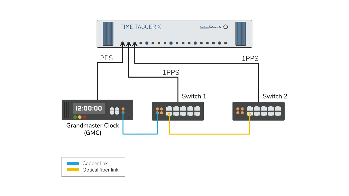
A typical 1PPS monitoring setup compares the selected edge of one or more DUTs with that of a reference 1PPS signal, typically the rising edge. The reference may be provided by a GNSS-disciplined receiver or oscillator, a local time/frequency standard, a grandmaster clock, or another timing source whose time scale, stability, uncertainty, and traceability are specified and sufficiently better than the DUT for the measurement being claimed. Each pulse edge is timestamped by the timing instrument, and the main measured quantity is the DUT-reference time offset for each nominal second.

Fixed delays in the reference and DUT signal paths are calibrated when absolute alignment is required, or treated as constant offsets when the goal is stability monitoring. From the resulting time-offset sequence, users can analyze absolute offset, epoch-to-epoch variation, drift, wander, holdover behavior, and recovery after reference changes. For long observation windows, the timing instrument’s time base must be sufficiently stable or referenced so that slow DUT behavior is not masked by measurement-system drift.

After the DUT, reference, selected edge, and calibration assumptions are defined, the main experimental challenges are:

Timing electronics single-shot jitter and time base: Beyond front-end bandwidth, the instrument itself introduces two additional error sources: single-shot timestamp jitter from its time-to-digital conversion and time-base drift over the observation window. Single-shot jitter sets a floor on how small a time-error excursion can be resolved on any one pulse. Time-base drift accumulates over longer windows and, unless the instrument’s own clock is stable or externally referenced, can be mistaken for slow DUT wander or holdover behavior.

Analog front-end bandwidth: For instruments that timestamp edges via a fixed voltage threshold crossing, a finite slew rate means the measured crossing time depends on the effective slope at the input comparator/trigger. Bandwidth limitation, attenuation, or conditioning that slows the edge reduces the signal slope at the trigger point, increasing noise-to-time conversion. Amplitude variation and threshold selection can also introduce threshold-crossing shifts, often described as time walk. Rigorous measurements, therefore, require a stable voltage threshold definition and sufficient front-end bandwidth so the “timestamped edge” is consistent across channels and setups.

Systematic delays and delay variation in distribution: Fan-out, level conversion, media conversion, and cabling introduce fixed latency plus potential delay variation, power-supply and aging effects. Fixed delays must be calibrated if absolute alignment is claimed; delay variation directly degrades stability metrics and must be bounded or characterized as part of the uncertainty budget.

Pulse integrity and association: A 1PPS monitor must distinguish valid pulses from missing pulses, extra pulses, double edges, or pulses outside the expected association window. These events are not ordinary jitter or wander; they indicate timing-chain integrity issues and must be recorded separately from steady-state offset statistics.

Multi-channel capability: For comparing multiple DUTs, simultaneous acquisition on one timing instrument is ideal because all channels share the same time base. If signals are captured on different instruments, their independent time bases introduce unknown relative offset and, more importantly, relative frequency/phase noise, which appears as artificial Time Interval Error (TIE) drift/wander between channels and is indistinguishable from DUT behavior unless the instruments are locked to a common reference and the inter-instrument offset/drift is characterized.

Swabian Instruments Time Taggers enable pulse-per-second monitoring by combining simultaneous multi-channel edge time-stamping (all channels referenced to the same internal time base) with a software stack designed for continuous acquisition, real-time visualization, and user-configurable analysis workflows.

Application Page

Frequency Stability Analysis

Role of timing electronics in Frequency Stability Analysis

查看更多内容