
Phase Noise Analysis
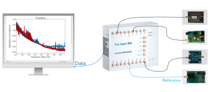
What Is Phase Noise Analysis, and Why Does It Matter?
Phase noise is random fluctuations of the phase of an otherwise periodic signal, commonly represented in the frequency domain as sidebands around the carrier; that is, it quantifies phase deviation relative to an ideal periodic reference. It is usually reported as single-sideband phase noise, L(f), a relative spectral density. Formally, IEEE Std 1139 defines , where is the spectral density of phase fluctuations, expressed in 1.
For sufficiently small phase deviation, has the familiar interpretation of the power in one sideband per 1 Hz bandwidth, normalized to the carrier power. This is why is conventionally expressed in dBc/Hz: “dBc” means decibels relative to the carrier power, and “per Hz” indicates normalization to a 1 Hz bandwidth. For example, -100 dBc/Hz at 10 kHz offset corresponds to sideband power 100 dB below the carrier in a 1 Hz bandwidth centered 10 kHz away from the carrier.
This sideband-power interpretation is useful, but it should not be applied unconditionally to a direct measurement of the RF spectrum. The measured sidebands can contain contributions from both amplitude-modulation (AM) noise and phase-modulation (PM) noise, and sideband power alone does not distinguish between them. The implications of this ambiguity for direct-spectrum measurements are discussed below.
Bandwidth-limited integrated timing jitter is obtained from by converting the spectrum to linear units, integrating over a specified offset-frequency range [f₁, f₂], and converting the resulting RMS phase fluctuation to time units using the carrier frequency.
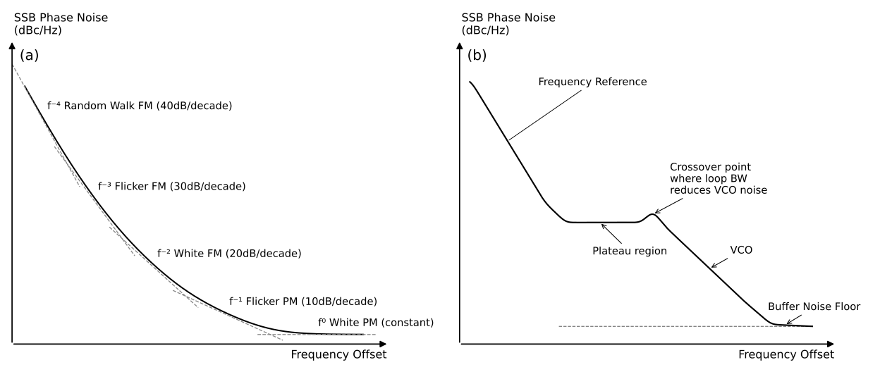
Figure 2. (a) Sketch of oscillator phase noise mechanisms. Phase noise arises from random noise sources (thermal, shot, flicker) that dominate over different offset-frequency ranges depending on the oscillator design and technology, producing multiple characteristic power-law regions. (b) Sketch of PLL phase noise mechanisms. Output phase noise results from different circuit elements’ contribution: the reference dominates at low offsets, a plateau from the phase detector and divider follows, some peaking occurs near the loop bandwidth, and the VCO’s own noise, present throughout but suppressed within the loop bandwidth by the loop filter’s roll-off, and the output buffer sets the noise floor at the highest offsets.
At the component level, phase-noise analysis is a core tool in oscillator and synthesizer design. The shape of over a broad offset-frequency range, rather than only its value at a single offset, provides information about the dominant noise processes. On a log-log phase-noise plot, as schematically shown in Figure 2a, regions with slopes of approximately –40, –30, −20, −10, and 0 dB/decade are commonly associated with Random Walk FM, flicker-FM, white-FM, flicker-PM, and white-PM noise, respectively 2. Narrow peaks, or groups of harmonically related peaks, can indicate deterministic disturbances such as power-supply coupling, digital switching, modulation leakage, or environmental interference. Identifying these features helps relate different parts of the spectrum to likely physical noise sources 3, compare oscillator designs, and derive design-relevant quantities such as integrated jitter 2 and short-term frequency stability 2 4.
In a phase-locked or synchronization system, the measured spectrum also shows how reference noise, oscillator noise, and control-loop dynamics combine, as schematically illustrated in Figure 2b. Below the effective loop bandwidth, the output typically follows the reference and other in-loop noise contributions, while the free-running oscillator or voltage-controlled oscillator increasingly determines the output noise above the loop bandwidth.
The crossover frequency, spectral roll-off, and any peaking around the transition can be compared with the intended loop bandwidth, loop-filter response, and damping. Discrete spurs may reveal reference feedthrough, power-supply disturbances, or periodic effects in the control path. These features help determine whether system performance is limited by the reference, the controlled oscillator, the loop design, or the measurement setup.
Because many electronic and photonic systems rely on a clock or frequency reference, phase noise can limit the performance of downstream modules and circuits by degrading sampling accuracy, modulation quality, spectral purity, synchronization margin, or coherent signal processing. No real source is ideal: thermal noise, flicker noise, device-specific noise processes, and phase-locked-loop dynamics all contribute to phase and frequency fluctuations 2. Characterizing these fluctuations enables consistent comparison of oscillators, synthesizers, and timing-distribution paths, supports jitter budgeting, guides choices such as loop bandwidth and filtering, and helps diagnose the origin of system-performance limitations.
Phase Measurement Architectures and Phase-Noise Interpretation
Phase-noise instruments estimate from measured sideband or phase-fluctuation data. The different measurement architectures mainly differ in how they obtain the phase information and in what limits the measurement floor.
In direct-spectrum measurements, the sidebands around the carrier are measured with a spectrum analyzer and normalized to the carrier power. This approach has several disadvantages compared to phase-detector- and FFT-based techniques: a swept spectrum analyzer captures one offset frequency at a time, so full-spectrum acquisition is slow, and this is only more difficult in a cross-correlation configuration, which relies on acquiring and processing long, simultaneous records rather than a single swept measurement. It also offers a limited dynamic range close to the carrier, and the analyzer’s own conversion oscillator adds further noise and instability of its own 2. Most fundamentally, as noted above, it measures total sideband power and cannot separate amplitude modulation (AM) noise from true phase noise 1, unlike the phase-detector-based and timestamp-based approaches described next.
In phase-detector-based measurements, often implemented with mixer-based or digital phase detection, the device under test (DUT) signal is compared with an internal or external reference after frequency translation, division, or multiplication if required; operating the detector in quadrature intrinsically suppresses much of the AM contribution 2. The relative phase fluctuations are converted into a baseband signal whose power spectral density (PSD) is estimated in software to obtain . Mixer-based phase detection can provide wide offset-frequency coverage and high sensitivity, but it requires suitable reference sources, analog phase-detection or frequency-translation stages, careful signal conditioning, calibration, and dedicated measurement hardware. This makes high-performance phase-noise analyzers accurate but complex and expensive. Cross-correlation architectures can further reduce uncorrelated measurement-channel noise by using two sufficiently independent measurement paths, at the cost of additional hardware and longer averaging time; correlated noise contributions do not average away 5.
The interpretation of the measured spectrum depends on the reference contribution and the measurement floor. If the reference path and instrument contribution are much lower than the DUT phase noise over the offset-frequency range of interest, the result can be interpreted mainly as DUT phase noise. If the reference, analyzer, or measurement channels contribute comparable noise, their contribution must be included in the uncertainty budget or reduced by the measurement architecture.
A timestamp-based approach uses a different method to obtain the phase samples. Instead of a dedicated analog phase detector, a timing instrument records recurring signal crossings and derives a stream of phase samples from deviations of the measured timestamps from an ideal or reference sequence. As in phase-detector-based measurements, the PSD of this phase-sample stream is then estimated in software to obtain . This approach is cost-efficient, flexible, and well-suited to multi-channel measurements. Its achievable measurement floor is mainly set by single-shot timestamping precision, signal quality at the selected crossing, edge slew rate, trigger-level sensitivity, and the stability of the reference or time base used to interpret the time tags. Because phase and timing error are related by , a given absolute timestamping uncertainty translates into proportionally more phase error at higher carrier frequencies: for a fixed timestamping precision, the achievable floor degrades by roughly 20 dB per decade increase in f₀.
The accessible offset-frequency range and resolution are set by the effective phase-sample rate and acquisition duration. With one valid timestamped edge per carrier cycle, for example, rising edges only, the Nyquist limit is f₀/2, where f₀ is the carrier frequency. Using both rising and falling edges doubles the phase-sample rate and extends the Nyquist limit to f₀, at the cost of doubling data throughput. Different edge types also introduce edge-dependent offsets or duty-cycle-related effects that must be considered when interpreting the resulting spectrum.
Common challenges in phase noise analysis include:
Measurement floor and instrument complexity. A central challenge in phase-noise analysis is separating the DUT contribution from the measurement-system noise floor. Reaching a low floor requires a carefully controlled measurement architecture, and cross-correlation requires two sufficiently independent measurement paths and longer averaging times. As a result, high-performance phase-noise measurements can require complex, costly, and less flexible instrumentation.
Offset-frequency range and resolution bandwidth. Phase noise is often characterized over several decades of offset frequency, from close-in regions where oscillator, control-loop, or timing-link dynamics shape the spectrum to far-from-carrier regions dominated by broadband noise or spurious tones. The relevant offset-frequency interval and effective resolution bandwidth must be defined because they determine which effects can be resolved and how spectra can be compared across instruments, DUTs, or measurement runs. For repeatable measurements, these settings must be documented and kept consistent, especially when comparing multiple devices or automating long measurement sequences.
Multi-Channel Comparison. Many practical phase-noise measurements involve more than one DUT, recovered clock, or timing-distribution output. Comparing these signals requires a common measurement basis, such as simultaneous acquisition on a shared time base. Within a synchronized system, acquiring both the distributed or recovered signal and the reference it is synchronized to, on two channels, allows their relative phase to be computed. Because the reference’s own phase noise appears in both records, it cancels in the difference to the extent that it appears identically in both, so the PSD of the relative-phase record characterizes mainly the noise added by the synchronization path itself, separate from the noise source being distributed.
The same logic extends across two independently synchronized systems: computing the cross-PSD between one channel per system reveals noise correlated between the systems, for example, from a shared upstream reference, while noise specific to each system is progressively suppressed by averaging. Either comparison, therefore, needs at least two channels, and as many as four when the within-system relative-phase measurement is itself cross-correlated between two independent instruments to remove that instrument’s own noise.AM-noise rejection in phase detection. Real signals carry amplitude-modulation (AM) noise alongside phase noise, and a measurement architecture must reject or otherwise separate the two 1. For instance, mixer-based phase detectors do this by operating in quadrature, often implemented with two mixers for I/Q sampling to hold the detector at that operating point 2; this adds analog hardware and calibration effort, and rejects AM noise only up to a given dynamic range.
Phase-noise and timing-workflow integration. Some measurement workflows require both frequency-domain phase-noise analysis and time-domain timing analysis. A user may need to measure , inspect time-error records, evaluate stability metrics such as Allan deviation derived from phase or time error 4, or monitor a pulse-per-second (1PPS) signal within the same workflow. In conventional setups, these tasks often require different instruments and separate analysis workflows, making automation, synchronization, and comparison more difficult. and Allan-type deviations illustrate the tradeoff well. Because time-domain stability metrics can be derived from the phase-noise PSD 4 but not the reverse, is the more complete description; however, the two converge at very different rates for long averaging times. An accurate modified Allan deviation out to 1000 s can typically be obtained from about an hour of acquisition when the instability is drift-dominated at that timescale, whereas accurately resolving down to the comparable 1 mHz offset from a single, non-cross-correlated measurement can take on the order of days. The additional offset-frequency resolution provided by is useful for identifying periodic errors and narrow spectral features, but it is generally unnecessary when the objective is only to characterize a drift-dominated noise regime. Deriving both from the same acquired time-tag stream lets a workflow default to the faster time-domain metric and fall back to the complete spectrum only when it is actually needed.
Advantages of Swabian Instruments’ Time Tagger for Phase Noise Measurement
Swabian Instruments’ Time Tagger builds on the timestamping approach introduced above, providing a software-defined workflow for phase-noise analysis of periodic signals. This approach is suited to carrier frequencies within the supported Time Tagger input and event-rate limits, which are model- and configuration-dependent and can extend into the hundreds of MHz. Key advantages of Swabian Instruments’ Time Tagger for phase-noise analysis include:
Use a Software-defined ReferenceClock. A periodic signal connected to a regular input channel can be selected as a software-defined ReferenceClock. The Time Tagger performs the time-to-digital-converter (TDC) measurement with respect to its internal oscillator; a software phase-locked loop (PLL) then evaluates the selected reference and rescales the time-tag stream before virtual channels and measurement objects process the data. For DUT phase-noise characterization, the selected reference must be sufficiently stable over the offset-frequency range of interest, or its contribution must be characterized. The same mechanism is useful for link characterization; for example, referencing a master node while analyzing a recovered clock on another channel. This software-defined approach is also more flexible than a traditional hardware reference input: a hardware clock input typically accepts only one or two specific frequencies within a narrow tolerance (for example, 10 MHz or 500 MHz, rejecting anything even a few percent off), interferes with the instrument’s self-calibration when the input is strongly correlated with the reference, and has a loop filter that is fixed at the factory. The software-defined ReferenceClock accepts arbitrary input frequencies and lets you tune the loop’s time constant to the reference at hand.
Reject AM Noise Inherently for Rectangular Signals. A timestamp-based measurement is affected by AM noise through a different mechanism than mixer-based quadrature detection: an amplitude change shifts the signal level at the fixed trigger threshold, which converts into a timing error scaled by the inverse of the slew rate at the crossing. Rectangular (square-wave-like) signals have a much steeper slew rate at the threshold than sinusoidal signals, which minimizes the time uncertainty in the analog-to-digital conversion in the presence of AM noise; mixers, by contrast, are best suited to sinusoidal signals. As a result, for rectangular signals, timestamping is inherently less sensitive to AM noise than mixer-based detection, without dedicated AM-rejection hardware. Any residual duty-cycle noise left behind is itself canceled by averaging rising and falling edge pairs, described next.
Cancel Correlated Trigger Noise by Averaging Rising and Falling Edges. Because low-frequency (flicker) noise on the input signal shifts the rising- and falling-edge trigger crossings in opposite directions, averaging a close rising/falling edge pair into a single combined timestamp cancels this correlated component while still improving uncorrelated (white) timing noise. The AM-to-timing conversion described above produces a similar signature: because rising and falling edges have opposite-sign slew rates, a given amplitude fluctuation shifts them in opposite time directions, so it shows up mainly as noise on the measured duty cycle rather than on the period. Averaging the edge pair cancels this duty-cycle noise as well. This is a distinct lever from simply using both edge types to double the phase-sample rate (discussed above): it trades sample rate for a lower noise floor rather than for an extended offset-frequency range.
Acquire Multiple Periodic Signals on a Common Time Base. Several DUT outputs or periodic sources can be recorded simultaneously on separate input channels. When acquired on the same Time Tagger, the signals share a common device time base, which simplifies relative phase-noise and timing comparisons. The available number of inputs is model-dependent; larger synchronized configurations can be built with the Synchronizer when higher channel counts are required. Parallel acquisition is valuable even when the units under test do not need to share a time base: measuring N devices at once on N channels reduces total test time by roughly a factor of N compared with testing them one at a time, which matters most when the required acquisition is long, as for the low-offset-frequency measurements described above. Combined with the cost-efficiency of a software-defined, multi-channel architecture, this makes the Time Tagger well-suited to high-throughput screening and quality-control testing after production, where cost-efficient throughput across many units is often more valuable than reaching the lowest achievable measurement floor on any single unit.
Support Automated and Reproducible Analysis Workflows. The Time Tagger software interface allows users to configure acquisitions, run phase-noise measurements, and export results. Native interfaces for Python, C++, MATLAB, and LabVIEW extend this into scripted, automated workflows, supporting customized analysis, automated stability testing, and repeatable measurements across multiple DUTs or long acquisition sequences.
Combine phase-noise analysis with related timing and frequency measurements. The same Time Tagger hardware and software ecosystem can support phase-noise analysis together with related measurements such as frequency-stability analysis (Allan deviation (ADEV), MDEV, TDEV, HDEV 4), time-interval measurements, frequency counting, jitter analysis, and 1PPS monitoring. This is useful when a workflow requires both frequency-domain phase-noise data and time-domain timing information: every derived quantity comes from the same simultaneously acquired time-tag stream, rather than from separate acquisitions on unrelated instrument platforms.
- Advanced cross-correlation workflow. For applications that require a lower measurement floor, the timestamping approach can be extended to a two-instrument cross-correlation workflow. In this configuration, the same periodic signal is acquired by two independent Time Taggers, synchronized by a common start trigger. Rather than averaging each channel’s own magnitude-squared spectrum, , as in a single-channel PSD, the workflow averages the cross-spectrum between the two independently measured phase records over many blocks. When the two acquisition paths are sufficiently independent, uncorrelated contributions between the measurement chains average toward zero, while phase fluctuations common to both records remain. This follows the same cross-spectral-averaging principle that underlies conventional dual-mixer phase-noise analyzers 2 5 and here extends the timestamp-based workflow to lower measurement-floor applications.
Frequency Stability Analysis
Role of timing electronics in Frequency Stability Analysis
Discuss your measurement
with our team
IEEE Std 1139-2022, IEEE Standard Definitions of Physical Quantities for Fundamental Frequency and Time Metrology-Random Instabilities, IEEE, 2022. ↩︎ ↩︎ ↩︎
E. Rubiola, Phase Noise and Frequency Stability in Oscillators, Cambridge Univ. Press, 2008 ↩︎ ↩︎ ↩︎ ↩︎ ↩︎ ↩︎ ↩︎ ↩︎
D. B. Leeson, “A simple model of feedback oscillator noise spectrum.” Proc. IEEE 54, 329–330 (1966) ↩︎
J. Rutman and F. L. Walls, “Characterization of frequency stability in precision frequency sources.” Proc. IEEE 79, 952–960 (1991) ↩︎ ↩︎ ↩︎ ↩︎
E. Rubiola and V. Giordano, “Correlation-based phase noise measurements.” Rev. Sci. Instrum. 71 (8), 3085–3091 (2000) ↩︎ ↩︎