Dynamic Light Scattering (DLS) Particle Size Analysis

Dynamic Light Scattering (DLS) is a widely utilized, non-invasive technique for analyzing the size distribution of particles suspended in liquid, particularly within the nanometer to submicron range. It relies on measurement of time-resolved intensity fluctuations of light scattered by particles undergoing Brownian motion in a liquid medium. These fluctuations are directly influenced by particle size: smaller particles diffuse more quickly and generate rapid fluctuations, while larger particles move more slowly, resulting in slower intensity changes. Autocorrelation analysis of the scattering intensity signal enables calculation of the translational diffusion coefficients of the particles and subsequent conversion into hydrodynamic diameters using the Stokes-Einstein equation. This provides accurate, real-time characterization of particle sizes in their native liquid environment without the need for labeling or extensive preparation. DLS is highly sensitive to nanoscale particles, positioning it as an indispensable tool across numerous scientific and industrial applications including pharmaceuticals, biotechnology, nanomaterials research, food technology, and cosmetic science.

Researchers routinely employ DLS to evaluate parameters such as particle size, distribution uniformity, colloidal stability, protein aggregation, polymer behavior, macromolecular interactions, and higher-order aggregates. DLS applications include evaluating therapeutic protein stability, tracking nanoparticle behavior in drug delivery systems, analyzing emulsion uniformity in consumer products, and detecting nanoplastics in aquatic environments.

One of the key advantages of DLS is its efficiency: it requires minimal sample volume, little preparation, and delivers results within seconds. Due to its particle size resolution across multiple orders of magnitude, DLS is the diagnostic tool of choice for identifying early signs of instability or contamination, vital for ensuring sample quality and performance over time.

Dynamic Light Scattering (DLS) relies on detection of light scattered by moving particles in liquid colloids. The scattered light from individual particles interferes with that from others, producing intensity fluctuations at the detector. Observing these fluctuations requires a highly monochromatic light source such as a laser. Moreover, the detector must be both fast and highly sensitive, since the scattered light can be extremely weak, especially for very small particles in dilute samples. Fortunately, detectors capable of single-photon sensitivity have been available for decades and are routinely used in DLS.

The mathematical foundation of DLS assumes that the observed intensity fluctuations are stochastic, as is the case when particle motion is dominated by thermally driven Brownian motion. In contrast, any organized motion in the sample, such as sedimentation or convection, usually introduces systematic distortions in the signal and must therefore be minimized when designing or carrying out an experiment.

While scattered light can, in principle, be detected at any nonzero angle, the rate of intensity fluctuations depends on the scattering vector $𝑞$, which is determined by both the scattering angle and the wavelength of the light. Typical measurement setups use side scattering at $90^\circ$ or back scattering near $180^\circ$. Some DLS instruments include a detector on a movable arm, which makes it possible to vary the observation angle and thus probe different scattering conditions.

When the temporal autocorrelation of the intensity fluctuations is analyzed, it becomes clear that larger particles produce slower fluctuations than smaller ones in the same liquid and conditions. This effect arises because larger particles diffuse more slowly, and it provides the fundamental link between the observed fluctuation dynamics and particle size in DLS.

The Autocorrelation Function in DLS

The Autocorrelation Function (ACF) is a central concept in Dynamic Light Scattering (DLS). It provides a framework for analyzing temporal fluctuations in the intensity of scattered light.

In a DLS experiment, the detector records scattered light as a sequence of individual photons, each separated by a varying time interval that reflects the random nature of scattering events. A precise timestamp is assigned to every detected photon, forming the basis for subsequent analysis.

To extract meaningful information about the underlying dynamics, these photon timestamps are processed mathematically by an autocorrelator. The outcome is the normalized intensity ACF, denoted as $g^{(2)}(\tau)$. This function measures how similar the signal is to itself after a delay time $\tau$. In other words, it quantifies the correlation between the light intensity at time $t$ and at a later time $t + \tau$.

Put simply: if a photon is detected right now, how much more (or less) likely is it that another photon will arrive after a delay $\tau$, compared to what would be expected from completely random arrivals?

While the ACF is primarily used to determine the particle size distribution, it also offers valuable insights into sample quality and measurement conditions. Several key characteristics of the ACF are outlined below. These aspects are especially important in dilute samples, where even minor inconsistencies can significantly affect the outcome of the analysis:

Intercept: reflects the coherence factor ($\beta$) and provides information about signal quality. It is worth noting that in DLS the intercept is an extrapolation of the recorded ACF to $\tau=0$ rather than actual value of $g^{(2)}(0)$ which is never measured directly.

• In practice, $g^{(2)}(0) - 1 = \beta$ should lie between 0 and 1.
• A high intercept (close to 1) indicates strong correlation and good experimental conditions (clean sample, proper alignment, suitable concentration).
• A low intercept suggests problems such as low particle concentration, weak scattering intensity, background noise, or misalignment.
• Intercepts that deviate strongly from this range (e.g., much lower than expected, or artificially higher than 1) usually indicate artifacts such as multiple scattering, detector saturation, afterpulsing, or contamination.

Decay Shape: of the ACF encodes the Brownian diffusion of the scatterers. When acquired under DLS-appropriate conditions (single scattering, stationarity, adequate SNR), it enables extraction of particle parameters, such as diffusion coefficient and hydrodynamic size, and their dispersity.

• A clean single-exponential decay indicates a monodisperse sample.
• A broadened or multi-exponential decay points to polydispersity, aggregation, or multiple populations of different sizes.

Decay Rate $\Gamma$: determines the characteristic timescale of particle diffusion.

• Smaller particles (with higher diffusion coefficients) produce faster decay (larger $\Gamma$), while larger particles lead to slower decays (smaller $\Gamma$).
• For a monodisperse system, the ACF shows a single exponential decay for which a mean decay rate can be extracted.
• In polydisperse colloids, the ACF is a weighted sum of exponentials for which a mean decay rate per component or a distribution of decay rates can be extracted.

Baseline $g^{(2)}(\tau \to \infty)$: indicates the long-time behavior of the ACF.

• Ideally, the baseline approaches 1, meaning that signals at widely separated times are uncorrelated.
• Deviations may result from number fluctuations (very dilute samples), aggregates or dust (slowly diffusing species), background light, or insufficient measurement time.

Determining the Particle Size

The ACF measured in a DLS experiment contains the key information needed to determine the particle size distributions¹. For monodisperse samples, this information can be extracted by fitting an exponential model. For polydisperse samples, more advanced approaches such as mathematical inversion are required to recover the full particle size distribution.

Field Autocorrelation Function: for a monodisperse suspension of spherical particles takes the form:

Equation 1. Characteristic exponential decay of the ACF for a monodisperse suspension. $\Gamma$ is the decay rate, and $\tau$ is the delay time.

Intensity Autocorrelation Function and Siegert Relation: In practice, DLS measures the intensity ACF, which is related to the field ACF through the Siegert relation:

Equation 2. Siegert relation and the form of $g^{(2)}(\tau)$ for a monodisperse system.

Here, the $\beta$ is a coherence factor (ranging between 0 and 1) and determined as an intercept value by extrapolating the ACF to $\tau=0$. $\Gamma$ is a decay rate that refers to the time scale of diffusion.

Translational Diffusion Coefficient $(D_{T})$: quantifies how rapidly particles move in the the solvent. For monodisperse particles, it is computed from the decay rate $\Gamma$ and scattering vector $q$ at which the ACF was recorded

Equation 3. Translational diffusion coefficient and the scattering vector.

Here, $n_0$ is a refractive index of a sample, $\lambda$ is a freespace wavelength of illuminating light, and $\theta$ is a scattering angle at which detector collects scattered light.

Hydrodynamic Radius $(R_{H})$: represents the radius of a theoretical hard sphere that diffuses through a solvent at the same rate as the observed particles. This value is not just a measure of the particle’s core size — it also includes contributions from any solvent layer or surface-bound structures. As such, $R_{H}$ is an effective size parameter that reflects the particle’s true behavior in its native liquid environment. It is calculated from the translational diffusion coefficient using the Stokes–Einstein equation:

Equation 4. Stokes-Einstein equation links the translational diffusion coefficient $D_{T}$ for a hard sphere of (hydrodynamic) radius $R_{H}$ at a given temperature $T$ (in Kelvin), solvent viscosity $\eta$, and the Boltzmann constant $k_{B}$.

When applying the Stokes–Einstein equation, it is important to account for the strong dependence of solvent viscosity on temperature. Even moderate changes in temperature can significantly affect the calculated radius.

Analysis Methods: Cumulants and Distribution algorithms

DLS measurements usually need to go beyond the previously discussed case of an ideal monodisperse distribution. Contemporary research requires direct measurement of polydisperse solutions, meaning that they contain a mixture of particles with various sizes. Since each particle size diffuses at its own characteristic rate, the observed ACF is a more complex function than a simple exponential decay. In DLS, particle size analysis is thus typically performed using two main approaches to interpret the ACF: Cumulants Analysis for monomodal samples², and distribution-based methods such as non-negative least squares (NNLS) or the CONTIN³ algorithms.

Cumulants Analysis applies a polynomial expansion to the logarithm of the ACF. From the first two terms of this expansion, it is possible to determine the intensity-weighted Z-average hydrodynamic radius and the polydispersity index (PDI), which provides a dimensionless measure of the breadth of the distribution². This method is straightforward and does not require prior assumptions about the underlying particle size distribution. However, it implicitly assumes that the distribution is monomodal. As a result, it yields only an average particle size and an estimate of polydispersity rather than a detailed distribution profile. The strength of cumulants analysis lies in its robustness and simplicity, which make it particularly useful for routine analysis of monomodal or nearly monodisperse systems. Its reliability, however, diminishes in the case of multimodal or highly polydisperse samples, where a single average value fails to capture the underlying complexity.

Distribution‑based algorithms extract size information by representing the ACF as a sum of weighted exponential decays, yielding a continuous distribution of decay rates. This procedure is equivalent to an inverse Laplace transform, which is mathematically ill-posed and requires stabilization through constraints. The non-negative least squares (NNLS) method addresses this by imposing a non-negativity constraint on all contributions, ensuring physically meaningful solutions but leaving the result sensitive to noise. The CONTIN algorithm goes further by introducing a smoothness constraint through regularization, which suppresses spurious oscillations and produces more stable, interpretable distributions. Although CONTIN is more computationally demanding and sensitive to the choice of regularization, it is particularly effective for resolving subtle or overlapping particle populations in polydisperse systems ³.

In summary, Cumulants Analysis offers a rapid and robust means of characterizing monomodal samples, yielding average size and polydispersity values that are often sufficient for routine measurements. Distribution-based algorithms, provide richer information and can reveal distinct particle populations within a sample, making them indispensable for the analysis of polydisperse or multimodal systems. Instruments that provide access to both approaches therefore offer users the flexibility to switch between high-throughput quality control and more detailed, research-grade characterization depending on the needs of the experiment.

Advantages of Multiple Angle Measurements

In DLS, the scattering angle plays a critical role in determining sensitivity to different particle sizes. Conventional instruments often operate at a single fixed angle, but the choice of angle directly influences resolution and data quality.

Forward scattering maximizes the contribution from large particles, which scatter predominantly in the forward direction. It is useful for samples where detecting larger particles or aggregates is important.

Side scattering at 90° provides a balanced compromise, offering good sensitivity across a wide size range with a favorable signal-to-noise ratio. This is the traditional geometry used in many DLS setups. Back scattering enhances sensitivity to small particles and, in modern implementations, reduces multiple scattering by probing only the near-surface region of the sample.

Modern multi-angle DLS instruments collect scattering data at several detection angles and combine the information into a single, angle-independent particle size distribution using Mie theory-based weighting. This approach is particularly beneficial for polydisperse or complex systems, where contributions from differently sized particles vary with angle. This approach is particularly advantageous for polydisperse or complex systems, where the relative scattering contributions of different particle sizes vary strongly with angle. By leveraging complementary data from multiple geometries, multi-angle DLS improves resolution, reduces angular bias, and increases confidence in the derived size distributions ⁴.

Historically, multi-angle measurements were only feasible in a sequential manner, requiring separate acquisitions at each angle, a process that was both time-consuming and instrumentally demanding. Recent advances in correlator electronics and the reduced cost of photon detectors now enable simultaneous multi-angle detection in compact and cost-effective instruments.

This capability provides a significant advantage in research, development, and Quality Assurance (QA) / Quality Control (QC) workflows, where both precision and reproducibility are essential. Measurements can be adapted to the specific properties of the sample — such as concentration, turbidity, and size distribution — yielding a more complete and reliable characterization of both monomodal and multimodal systems.

In traditional DLS systems, the Autocorrelation Function (ACF) of the scattered light intensity is computed using dedicated hardware correlators.

While this approach was historically the first commercially viable option, it imposes several limitations that can affect measurement accuracy, data reliability, and experimental efficiency. Key challenges include high sensitivity to contaminants, limited angular detection, restricted correlator capabilities, and detector afterpulsing artifacts.

Limited Correlator Functionality and No Access to Raw Data: The hardware correlator itself can impose fundamental limitations. Many conventional designs provide only a limited number of inputs, limited number of ACF values (channels), and offer minimal flexibility for advanced or customized data processing. These restrictions hinder the application of modern analysis techniques that could enhance resolution, compensate for noise, or extract additional information from the same dataset.

By design, hardware correlators process incoming photon events into the ACF prior to transmission to a computer for further processing. This completely prohibits the possibility to change key parameters such as correlation time intervals or the number of correlation bins after a measurement is complete. While this used to be necessary given limited data rates in older computing hardware, modern personal computers are more than capable to process and store each photon captured by a detector.

Sensitivity to Contaminants and Aggregates: Conventional hardware correlators are highly susceptible to noise introduced by dust particles, large aggregates, or other contaminants. Even rare contamination events produce irreparable intensity spikes that distort the ACF, biasing the size distribution toward larger diameters and compromising the accuracy of calculated particle sizes. Such distortions may lead to incorrect assessments of sample quality or stability, potentially delaying projects, disrupting workflows, or jeopardizing product development. Mitigation strategies typically involve manual, physical filtration and repeated measurements. However, these are prone to operator error, may be unsuitable for delicate samples, or increase the measurement time in an unpredictable fashion. Algorithmic post-processing can remove contaminated datasets, but necessitates longer acquisition times to maintain sufficient count rates, and may inadvertently discard valuable information, further impacting data integrity.

Angle-Dependent Scattering: Many DLS measurements involve anisotropic particles or polydisperse mixtures. In such cases, scattering intensity depends strongly on the detection angle. Larger particles or specific size fractions may dominate the scattering signal at certain angles, masking weaker contributions from other populations. Traditional DLS setups frequently measure at a single fixed angle, or sequentially across a small number of angles. For complex samples, single-angle acquisition can obscure subpopulations entirely. Sequential multi-angle measurements require repeated runs, increasing the risk of contamination, temperature drift, and experimental variability while extending overall acquisition time.

Afterpulsing in Detectors: Although afterpulsing is a detector-related artifact rather than a limitation of the correlator itself, it remains a common issue in DLS systems that employ single-photon avalanche diode (SPAD) detectors. Afterpulsing originates from charge carriers that become trapped in defect states within the semiconductor structure of the SPAD. During an avalanche event triggered by a photon, some of these carriers are captured in trap states and released later, producing spurious counts that mimic genuine photon arrivals.

The statistical properties of afterpulsing introduce an additional, nearly exponential decay component in the ACF at short delay times, typically for $\tau < 1$ µs. This effect is particularly detrimental in backscattering geometries, where the true diffusion-related intensity fluctuation rates are fast and thus overlap inseparably with the afterpulsing signal. If left uncorrected, afterpulsing degrades the accuracy of particle size determination.

A widely adopted method to mitigate this problem is the pseudo cross-correlation approach, in which the collected light is split and directed onto two identical detectors. By cross-correlating the signals from both detectors, the genuine diffusion-related correlation is preserved while the uncorrelated afterpulsing artifacts are effectively suppressed.

Hardware correlators are therefore falling behind the next-generation particle sizing platforms which incorporate high-speed, high-precision timing electronics capable of timestamping individual photon arrivals. Access to raw photon data enables flexible, experiment-specific post-processing, including complete storage of photon data, advanced noise filtering and customized correlation analysis. For anisotropic or polydisperse samples, the ability to collect and process scattering data from multiple angles simultaneously is particularly valuable. Multi-angle, time-resolved acquisition improves resolution, reveals otherwise hidden size populations, and enhances robustness across diverse sample conditions and bridging the gap between high-throughput quality control and advanced particle characterization.

Swabian Instruments provides two distinct pathways for enhancing Dynamic Light Scattering (DLS) experiments.

Replacing a Conventional DLS Correlator with a Time Tagger

For researchers designing custom systems, Swabian Instruments advances existing and new DLS configurations by replacing dedicated hardware correlators with high-performance timing electronics, also known as Time Taggers.

Time Taggers were originally developed for Time-Correlated Single Photon Counting (TCSPC) owing to their ability to record photon arrival times with exceptional precision and generate histograms from timing differences. In the context of DLS, these devices timestamp each detected photon with picosecond accuracy, allowing correlation functions to be computed entirely in software. This approach delivers flexibility in data analysis in real-time or by storing these events for post-acquisition processing tailored to the specific needs of the experiment. The advatanges of Swabian Instruments’ Time Tagger as a correlator include:

Access to Raw Data and Real-Time Analysis: The accompanying software enables rapid correlation calculations, real-time data inspection, and full access to the photon arrival stream. This capability supports the immediate detection and filtering of artifacts caused by transient intensity fluctuations from contaminants, aggregates, or particle clusters. As a result, correlation functions can be corrected in real time, improving the reliability of particle size measurements, particularly for complex or evolving samples.

High Precision and High Throughput: Swabian Instruments Time Taggers provide picosecond timing resolution, ensuring accurate temporal characterization of the scattered signal. Their high count-rate capacity makes them well suited to the intense photon streams often encountered in scattering experiments with multiple detectors.

Data Reliability through Multi-Angle Simultaneous Measurement: With multiple fully independent input channels, a Time Tagger can acquire signals from several scattering angles at the same time. This allows real-time consistency checks across angles, enhancing accuracy in samples with contaminants, aggregates, or broad size distributions.

Replacing a conventional correlator in a custom DLS setup with a Swabian Instruments Time Tagger provides a cost-effective and straightforward upgrade with immediate benefits in measurement flexibility, precision, and data quality. The timestamp-based, software-driven approach enables raw data storage, advanced post-processing, simultaneous multi-angle acquisition, and enhanced robustness against noise. These capabilities are particularly valuable for analyzing polydisperse, anisotropic, or aggregation-prone samples, where conventional correlator limitations can hinder accurate characterization.

DLScat: A Turn-Key Solution with the Benefits of Time Tagger 20

DLScat is a fully integrated DLS platform built around Swabian Instruments’ Time Tagger 20. In this system, the Time Tagger 20 functions as both the high-precision time-stamping engine and the photon correlator, ensuring accurate measurement of the Autocorrelation Function (ACF) and photon arrival statistics. By combining this timing technology with carefully selected optical and detection components, DLScat is designed to deliver precise and reproducible particle size measurements. The system offers high accuracy, flexibility, and full data transparency through the following core elements:

High-Stability Laser Source: DLScat employs a highly monochromatic and stable laser to ensure consistent scattering with excellent signal-to-noise ratio (SNR) and long-term stability. Visible-wavelength lasers are often preferred for protein sizing and nanoparticle characterization, as they provide a suitable balance between scattering efficiency and sample compatibility. Users may also select custom wavelengths to match the optical properties of their samples or to minimize absorption and fluorescence background.

High-Performance Single-Photon Detectors: The standard configuration uses fiber-coupled Single-Photon Avalanche Diodes (SPADs), offering low dead time, high quantum efficiency, and low afterpulsing. These properties are essential for measuring weakly scattering samples such as dilute proteins or sub-50 nm nanoparticles.

Multi-Angle Simultaneous Dynamic Light Scattering (MASDLS) Detection: DLScat measures simultaneously at multiple scattering angles to improve accuracy in size characterization and provide internal consistency checks, particularly important for polydisperse or anisotropic samples. The system can operate measure simultaneously at up to 5 angles 20°, 69°, 90°, 111°, and at 157°. Such configuration enables more reliable determination of particle size distributions and better resolution of polydispersity or structural heterogeneities in complex samples. The backscattering angle in the DLScat system includes two detectors to mitigate afterpulsing by calculating the cross correlation instead of the auto correlation value of the signal.

Software-Defined, Real-Time Processing: Leveraging the Time Tagger 20 as an efficient, high-throughput correlator, DLScat can acquire photon arrival times from multiple detectors simultaneously and stream them to a PC. Real-time computation and visualization of ACF allow users to adjust measurement conditions on the fly. The unique DLScat software provides direct access to raw time-tagged data from each angle, supports a range of analysis algorithms, and includes tools to suppress artifacts such as intensity spikes caused by dust or transient aggregates. This also enables detailed studies of kinetic processes in samples that change with time.

User-driven, research-enabler, easy to use: DLScat is built with the user in mind, pairing intuitive software with plug-and-play hardware so one can go from sample to high-quality data in minutes without requiring specialized training or delicate alignment. DLScat offers advanced measurement control capabilities and optimization for a variety of adjustments: tailor detector/angle configurations, choose analysis paths (cumulants or CONTIN), and access raw time tags, correlation curves, and complete metadata - no black boxes, no lock-in. Flexibility extends to optics and detection, including custom laser wavelengths and export of raw photon streams for advanced analysis. Guided by a user-driven roadmap and frequent software enhancements, DLScat is easy on day one.

To summarize, a conventional hardware correlator can be easily replaced with a Time Tagger, which records photon arrival times with picosecond precision and enables software-defined correlation analysis. For those seeking a complete solution, the DLScat offers a turnkey DLS platform for real-time, multi-angle, and software-defined particle size analysis. By combining the timing precision of the Time Tagger 20 with carefully engineered optical components including laser and detectors. This integration enables high-resolution measurements, improved reliability for polydisperse samples, and unrestricted access to raw experimental data, expanding the capabilities of particle size characterization techniques.

Swabian Instruments’ Time Tagger technology provides a significant leap in precision, flexibility, and data accessibility for DLS experiments. We offer two pathways to integrate this capability: (1) DLScat as a complete, turnkey platform and (2) Integration of Time Taggers within custom-built flexible DLS setups. In both approaches, replacing a conventional DLS correlator with a Time Tagger enables low timing jitter, minimal dead time, high data transfer rates, and direct access to raw photon arrival data. These features support more accurate, versatile, and transparent measurements.

By recording time-stamped photon arrivals across multiple detection angles simultaneously, Time Taggers enable software-defined correlation functions that can be adapted to specific experimental requirements. This approach offers high temporal resolution, precise size determination, and extensive customization in both data acquisition and analysis workflows. Built-in tools for filtering out transient intensity spikes from dust or aggregates further improve data quality, enabling cleaner correlation functions and more reliable particle size distributions. This approach lays the foundation for new possibilities in DLS data interpretation and experiment control and ensures a future-proof investment for all application scenarios.

For researchers seeking an out-of-the-box solution, the customized DLScat integrates all the benefits of Time Tagger technology into a streamlined DLS solution. The system features a clear separation between electronic and optical components, enabling extensive experimental customization in a compact form-factor. The electronics module includes the Time Tagger correlator, optical attenuators, and single-photon detectors. The optical setup, which can be independently configured by the user, allows optimization for specific measurement environments. Researchers can choose laser sources at different wavelengths, adjust optical alignment, integrate temperature control, and connect their custom optical arrangement to the electronics module via optical fibers coupled to the detectors. This modular design ensures compatibility with diverse sample types and environments, including in-situ experiments alongside Small-Angle Neutron Scattering (SANS) or Small-Angle X-ray Scattering (SAXS), in-situ irradiation studies, glove box operations, and other specialized setups. The modular design results in a versatile DLS platform that retains the precision, resolution, and real-time analysis capabilities of the DLScat system while expanding its application space far beyond conventional configurations.

Whether incorporated into a customized setup or used in its turnkey DLScat configuration, Swabian Instruments’ technology extends the capabilities of particle size analysis beyond the limits of traditional DLS, thus enabling faster, clearer, and more reproducible insights into particle behavior.

Measuring multi-modal particle sizes using DLScat

measuring-multi-modal-particle-sizes-using-dls-cat.pdf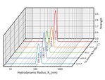

Introduction to Particle Sizing with DLScat

introduction-to-particle-sizing-with-dls-cat.pdf